Exploring LoRA — Part 1: The Idea Behind Parameter Efficient Fine-Tuning and LoRA | by 3pi | inspiringbrilliance

Table of contents

What is the need for fine-tuning?

Pre-trained large language models are trained extensively on large amounts of material from the Internet, resulting in superior performance on a wide range of tasks. Nonetheless, in most real-world scenarios it is necessary for the model to possess expertise in a specific specialized area. Many applications in natural language processing and computer vision rely on the adaptation of a single large-scale pre-trained language model for multiple downstream applications. This adaptation process is often achieved through a technique called fine-tuning, which involves customizing the model for a specific domain and task. Therefore, fine-tuning models is critical to achieving the highest levels of performance and efficiency on downstream tasks. Pre-trained models provide a solid foundation for a fine-tuning process that is specifically tailored to solve the target task.

What is the traditional way of fine-tuning?

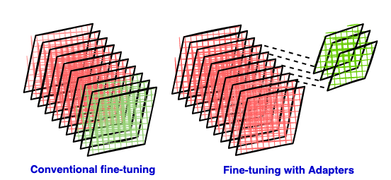
In traditional fine-tuning of deep neural networks, modifications are applied to the top layers of the network, while lower layers remain fixed or “frozen.” This is necessary because the label space and loss function of the downstream task are often different from those of the original pre-trained model. However, a significant drawback of this approach is that the resulting new model retains the same number of parameters as the original model, which can be quite large. Nonetheless, when using contemporary large language models (LLMs), creating separate complete models for each downstream task may not be efficient.

In many cases, the top layer and original weights are trained together. Large language models (LLMs) have reached such enormous scale that fine-tuning even a single layer, let alone the entire model, requires significant computational resources and can be prohibitively expensive. Take Llama 3.1-8B as an example: it contains 32 layers, excluding embedding and normalization layers, with approximately 218 million parameters per layer (combining all projection/attention and MLP layers). Traditional fine-tuning, even if limited to the last layer, can become a costly endeavor. At the end of this blog we will see how to improve this situation.

How can fine-tuning be made efficient?

Many people try to alleviate this situation by learning an additional set of parameters for each new task. In this way, in addition to the pre-trained model for each task, we only need to store and load a small number of task-specific parameters, which greatly improves the operational efficiency during deployment. This is one of the Parameter Efficient Tuning (PEFT) methods, which focuses on fine-tuning only external modules called adapters. This approach significantly reduces computational and storage costs.

The advantages of using parameter-effective methods for fine-tuning can be reflected in two aspects:

• Regarding disk storage: fine-tuning adapter modules with only a limited number of additional parameters requires only storing the adapter for each downstream task. This significantly reduces the storage space required for the model. It raises the question of whether it is really necessary to maintain a complete additional copy of LLaMA for each different subtask.
• Regarding RAM: While precise measurements of memory usage take into account factors such as batch sizes and various buffers required during training, general memory requirements are approximately four times the model size. This takes into account gradients, activations and other elements for each parameter. Fine-tuning smaller parameter sets alleviates the need to maintain optimizer state for most parameters. During the forward pass, frozen layer weights are used to calculate the loss without storing local gradients, eliminating the need to save the gradients of these layers, thus saving memory. During the backward pass, the weights of the frozen layers remain unchanged, which also saves computing resources and RAM because no computation is required to update these weights.

How to fine-tune with fewer parameters?

Li et al.² and Agajanyan et al.³ shows that the learned over-parameterized model actually exists in lower intrinsic dimensions⁸. This line raises several interesting questions: What are the intrinsic dimensions (ID) of the model? What is an over-parameterized model? What are the dimensions of the model? What is the dimensionality of the objective function? If the ID is so low, why do we have such a huge network in the first place? What is the relationship between ID and fine-tuning, and how to find the ID of a model? These issues will be discussed in detail this and accompanying article.

To pave the way for our discussion about LoRA, here is a quick summary –

1. While a deep network may have a large number of parameters (e.g. “n”), only a small subset of them (e.g. “d”), where d<, truly influences the learning process². The remaining parameters introduce additional dimensions to the solution space, simplifying the training process. The abundant solution space facilitates smoother convergence. 'd' represents what they call the model's ID for that particular task.
2. Larger models are easier to fine-tune because they can learn better representations of the training data and tend to have smaller intrinsic dimensions (ID).
3. Models that have been pretrained for a longer period of time are easier to fine-tune. Extended pre-training effectively compresses knowledge and reduces intrinsic dimensionality (ID)3.

What are adapters and how are they used for fine-tuning?

Adapter module, see the paper for details Holsby et al.1, involves making subtle architectural adjustments to repurpose pre-trained networks for downstream tasks. The adapter module is a dense layer (full size matrix) is introduced between the existing layers of the pretrained base model, which we refer to here as the “adopted layer” article⁴.During the fine-tuning process, the weights of the original network remain frozen, allowing only new adapter layers to be trained, allowing the original network’s unchanged network parameters to be shared across multiple tasks. exist Part 2we will explore how adapters are integrated into the overall architecture including the base model.

Adapter modules have two key features:

• Compact size: The adapter module has a relatively smaller number of layers than the original network. This is crucial because the main purpose of the adapter is to save space by storing fewer parameters for each downstream task, rather than duplicating the entire base model.
• minimal disruption: Initialization of adapter modules should be designed to minimize interference with training performance in early stages. This allows the training behavior to be very similar to the original model, while gradually adapting to downstream tasks.

What is LoRA?

LoRA (low-rank adaptation) is an adapter technique that involves inserting a low-rank matrix as an adapter. The authors of LoRA⁶ assume that adapter modules (new weight matrices adapted to the task) can be decomposed into low-rank matrices with very low “intrinsic rank”. They propose that large, pre-trained language models have lower “intrinsic dimensionality” when adapted to new tasks.

The idea behind low-order adaptation

Consider a matrix, denoted A, whose dimensions p x qwhich contains certain information. The rank of a matrix is ​​defined as the maximum number of linearly independent rows or columns it contains. A concept often introduced in schools is that rankings can be easily determined from the ladder form of a matrix. When the rank of matrix A (denoted as r) is smaller than p and q, such a matrix is ​​said to be “rank deficient”. This means that the full size matrix (p x q) does not have to convey all the information because it contains a lot of redundancy. Therefore, fewer parameters can be used to convey the same message. In the field of machine learning, matrices with lower order approximations are often used to carry information in a more concise form.

The purpose of the low-rank approximation method is to approximate matrix A with another lower-rank matrix. The goal is to identify matrices B and C, where the product of B and C is approximately A (A_pxq ≈ B_pxr × C_rxq), and both B and C have lower grades than A. r And determine B and C accordingly. p x r + r x q << p x q indicating that the space required to store the same information is significantly reduced. This principle is widely used in data compression applications. You can choose one r Less than the actual ranking of A, but constructing B and C in such a way that their product is approximately similar to A, effectively capturing the basic information. This approach represents a balance between preserving important information and managing spatial constraints in data representation. The reduction in the number of rows and columns that encapsulate the essential information in a data set is often referred to as the key characteristic of the data. Singular value decomposition (SVD) is a technique used to identify matrices B and C given a matrix A.

The authors of LoRA assume that the adapter (weight update matrix) has a lower intrinsic hierarchy, meaning that the information contained in the matrix can be represented using fewer dimensions than the adapter matrix/layer of the base model.

Instead of decomposing the selected adapter matrix via SVD, LoRA focuses on learning low-rank adapter matrices B and C for a given specific downstream task.

In our example A_pxq = W_2000x200, B = lora_A and C = lora_B. We use low-dimensional representations to approximate high-dimensional matrices. In other words, we try to find a (linear) combination of a small number of dimensions in the original feature space (or matrix) that captures most of the information in the original matrix. choose smaller r Resulting in more compact low-rank matrices (adapters), which in turn require less storage space and involve fewer computations, thus speeding up the fine-tuning process. However, the ability to adapt to new tasks may be compromised. Therefore, there is a trade-off between reducing spatiotemporal complexity and maintaining the ability to efficiently adapt to subsequent tasks.

in conclusion

Looking back at the example at the beginning of this blog, using LoRA to fine-tune Llama 3.1–8B at r = 2 reduces the number of trainable parameters to only 5 million – a significant saving compared to traditional storage and computational requirements. Storage and compute requirements are fine-tuned.